Collection of home made microstrip passive RF components

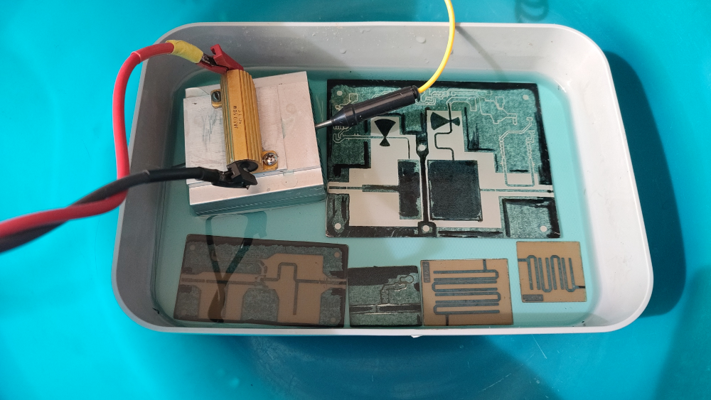
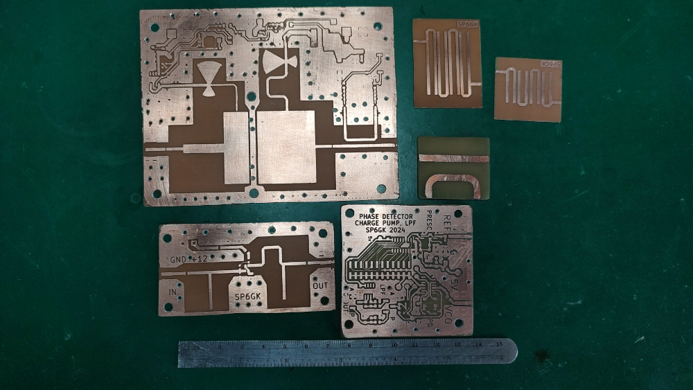
As a student, I have access to AWR Designer, a powerful tool for RF design and simulation made by Cadence. I present some results of my personal projects, which I have done mainly as a self-learning exercise with the possibility of using these parts later on. All my microstrip boards are made at home using a laser printer and iron for thermal transfer onto a laminate, which is then etched in a sodium persulfate solution. I am using double-layer laminates with 35 μm thick copper and 1.6 mm or 0.6 mm FR-4 substrate. I publish the results of the projects not the PCBs since they are made using educational version of AWR Designer. I hope the results will be useful to someone in evaluation of their results.

Filters

1.25 GHz Hairpin filter

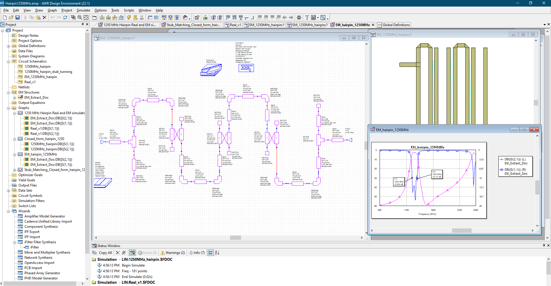
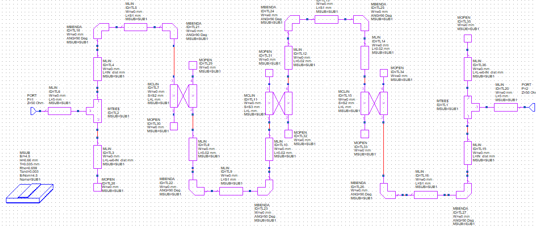
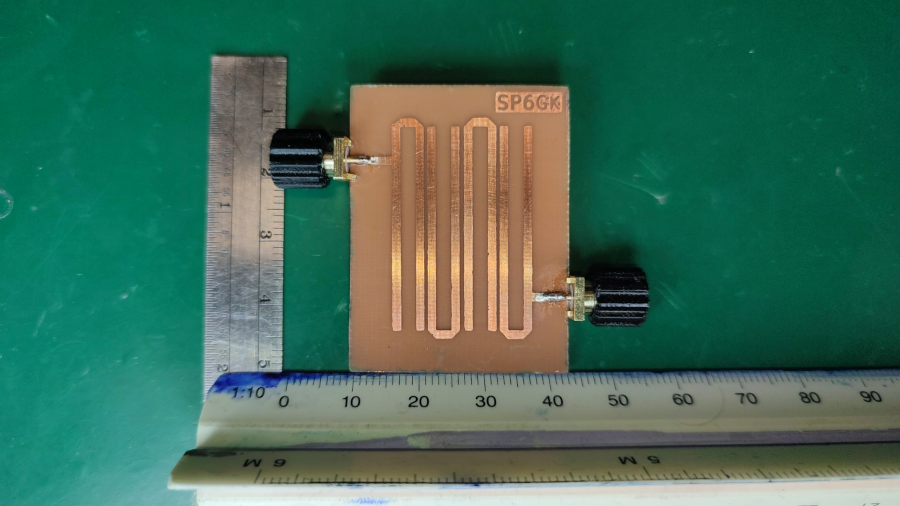
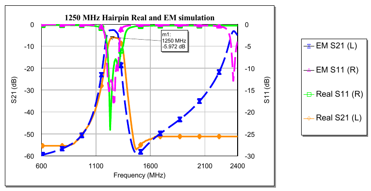
This filter was designed to cover the 23 cm amateur radio band. It uses four hairpin resonators. The figure below shows the insertion loss and return loss for both the EM simulation in AWR Designer and the measurement done on the real filter. It can be seen that the passband is very similar in both cases. The return loss is not as good as the simulation predicted, but it is acceptable and, in most of the band, it is below -10 dB. The insertion loss is almost -6 dB, which is higher than in the simulation where only -2.6 dB was observed. This result is not great when compared to SAW or other cavity filters, but the cost of implementation is very low and the attenuation is greater than -50 dB in the stopband, which is quite good. This filter could be used at the output of the TX mixer or between the LNA and RX mixer. The bandwidth (-3 dB) spans from 1215 MHz to 1333 MHz, so 118 MHz. The design of the filter started with a bandwidth of only 70 MHz, while in EM simulation the measured bandwidth was 107 MHz, which is closer to the desired 70 but still higher. This also shows that the EM simulation is closer to reality when compared to the filter synthesis tool, which is based on lumped model simulation. This result is, of course, to be expected since the lumped model in this case is only an ideal case and an approximation of the real structure. The real filter achieved a Q factor of 10.59, while the EM simulation yielded a Q factor of 11.68, so slightly better. For substrate information, the following parameters were used:

• H = 0.66 mm (Substrate height)
• T = 0.035 mm (35um copper trace)
• Rho = 0.698 (Based on conductivity of copper in TX line tool)
• Tand = 0.003 (Tangent loss of FR4)
• Er = 4.5 (Dielectric constant of FR4)

In simulation filter was simulated with 0.05mm grid and AXIEM simulator.

2.4 GHz Hairpin filter

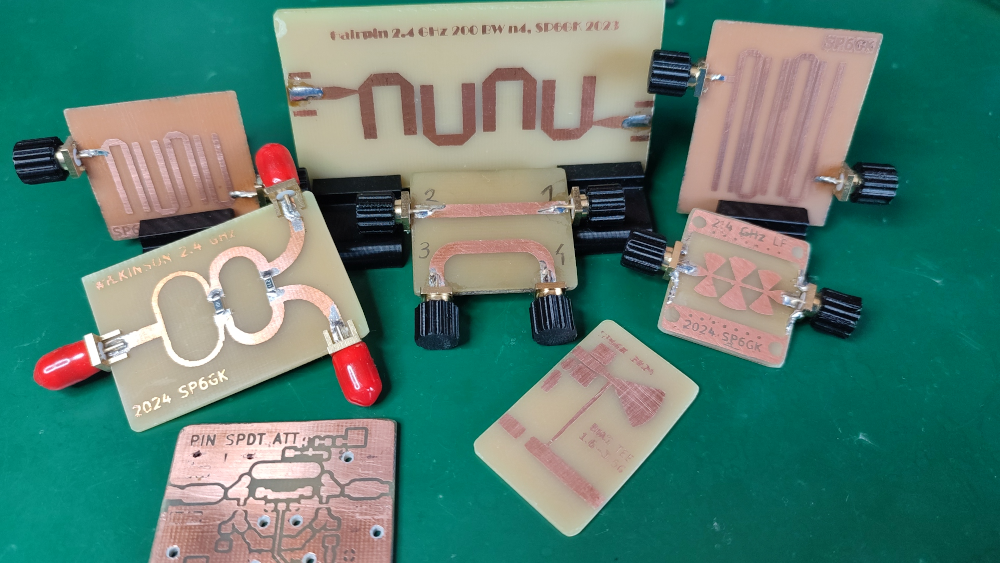
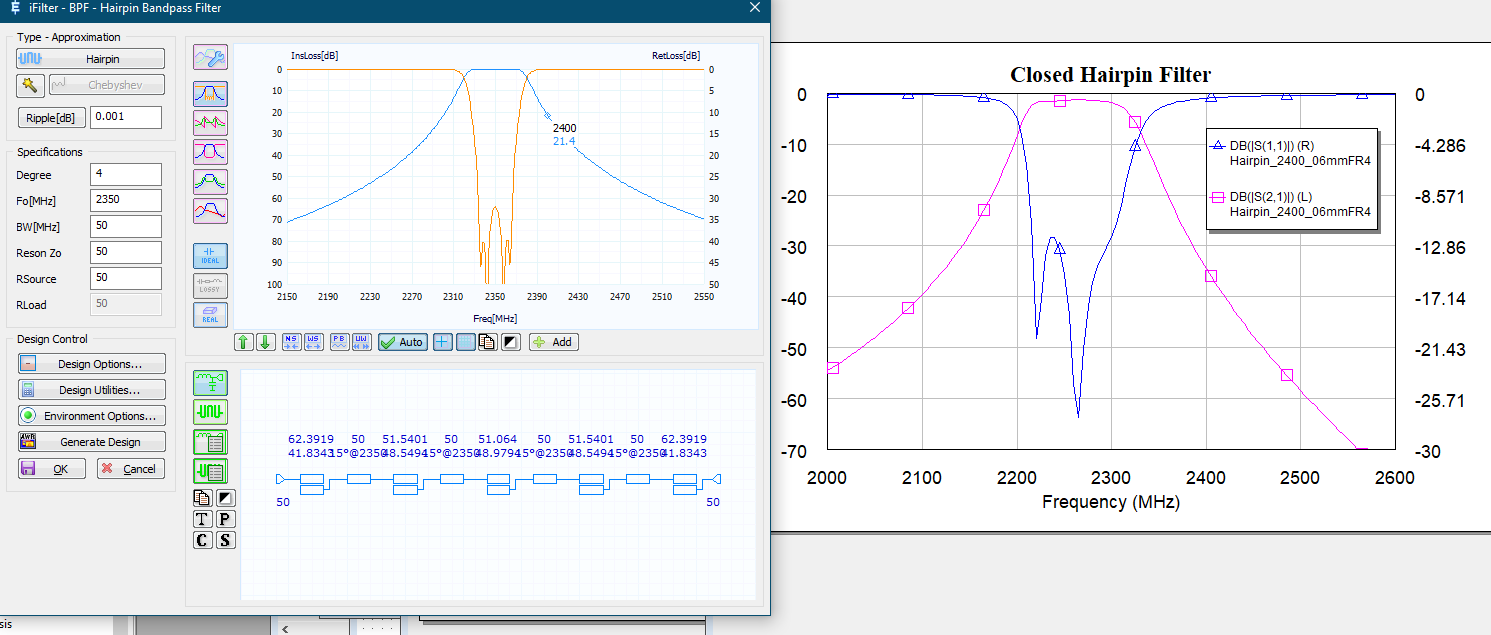
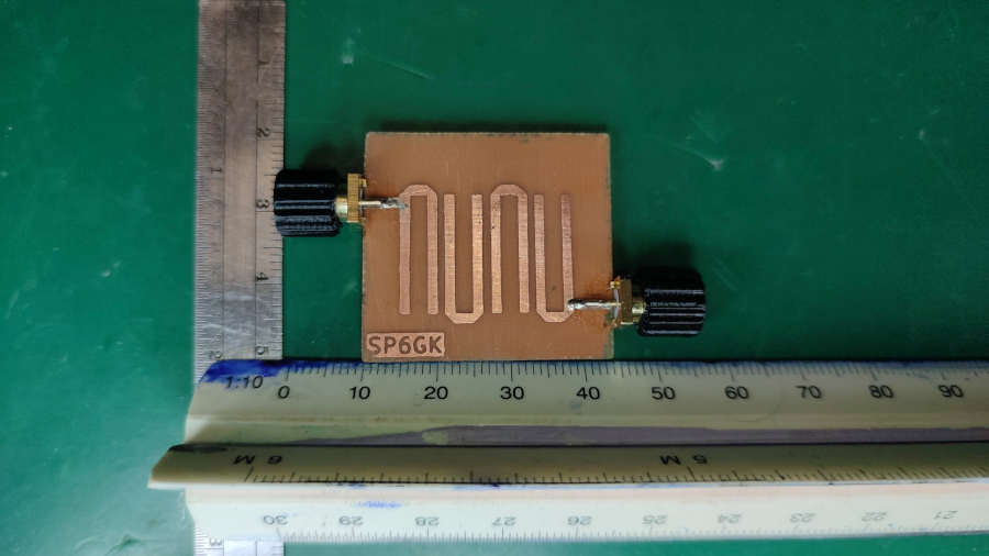
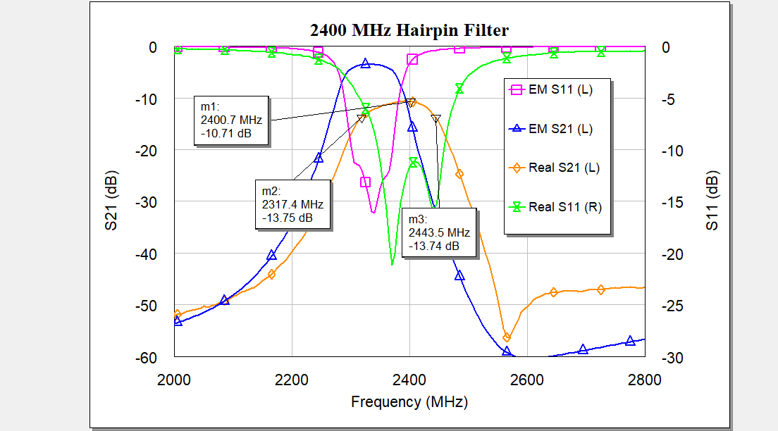
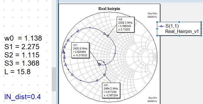
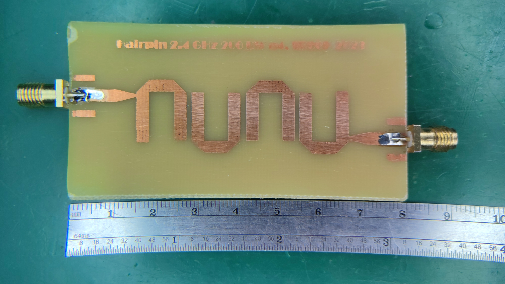
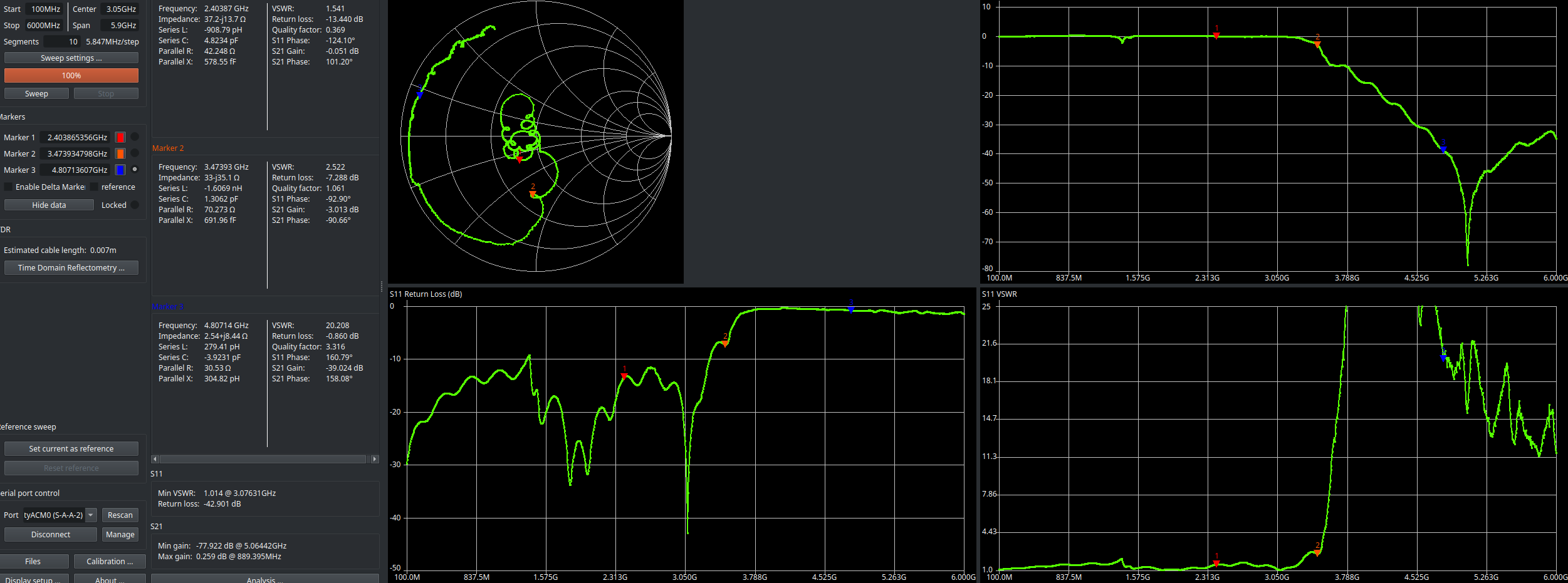
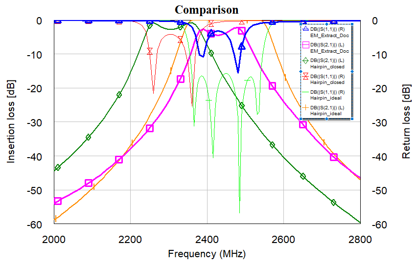
This filter was designed on the same substrate as the 1.25 GHz hairpin filter. However, it's my second revision of the hairpin filter for 2.4 GHz, but I will write more about that later on. For now, let me focus on the parameters that I have obtained in EM simulation and the real filter. In the filter design tool, the bandwidth of 50 MHz was chosen, and the center frequency was set to 2350 MHz. Why not exactly 2.4 GHz? Well, from my previous attempt, I expected that the real filter would shift up in frequency by about 50 MHz. As can be seen from the plot below, the center frequency was achieved; however, the insertion loss is very high, more than 10 dB. The bandwidth is also wider than in the EM simulation. This indicates that the Q factor of the resonators was lower in reality than in the simulation. The insertion loss in the real filter is acceptable and stays below -7 dB throughout the passband, and is more than -10 dB from 2350 MHz to 2450 MHz. The -3 dB bandwidth is 126 MHz in the real filter and 93 MHz in the EM simulation, yielding Q factors of 19.04 and 25.8, respectively. The same parameters for the substrate were used except for the dielectric constant, where a value of 4.4 was entered. This is because, despite being "constant," the Er does decrease with frequency for FR4. The exact value is not known for this laminate, so take this as an estimate. Since tangent loss can also increase, changing the value to something higher than 0.003 might be a good idea as well.

2.4 GHz Hairpin filter (old version)

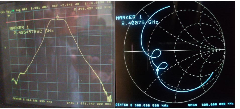
This was my first attempt at making a bandpass filter on a microstrip. It did work however, the center frequency was significantly shifted to the right. It also used a 1.6 mm thick PCB, so the traces are very wide to maintain the low impedance.

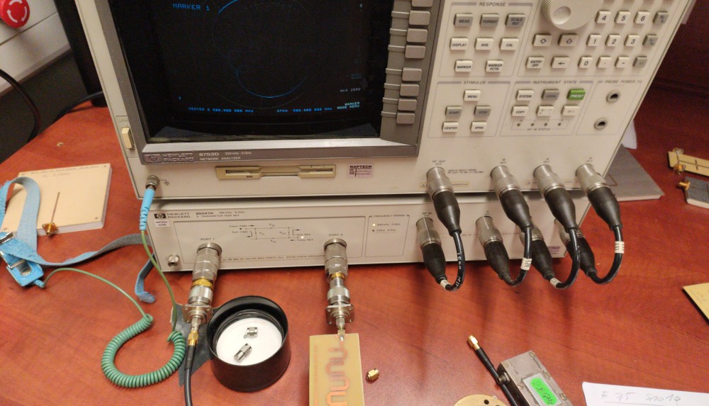
Using the HP vector network analyzer at my uni I have determined the following parameters.

Parameter	EM simulation	Measured	Unit
Insertion loss	4.26	6.97	dB
Fc	2.450	2.495	GHz
3 dB bandwidth	130	190	MHz
50 dB bandwidth	761	781	MHz
Attenuation slope	0.1459	0.1102	dB/MHz
Attenuation at 2 GHz	53	51	dB
Q	18.46	13.13	N/A

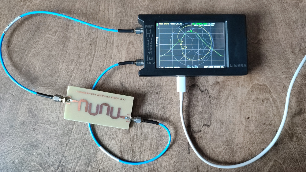
I was able to measure this filter using both modern and cheap Lite VNA64 and an old HP VNA at my university. To be honest I would love to have such an instreument in my own lab but the only significant difference nowadays seems to be the dynamic range. Anyway here is a comparison of results between two instruments: Overall the LiteVNA has produced very similar results in S21 measurement. For example at 2 GHz marker the HP instrument noted lower insertion loss of only 3 dB which is not that significant above 50 dB of dynamic range. The insertion loss at 2.5 GHz is also comparable, -6.27 dB (LiteVNA) vs -6.97 dB (HP). For a 2.4 GHz the HP measures IL of -9.7 dB and the LiteVNA measures -8.7. When it comes to return loss the devices differ a little bit in their precision but again LiteVNA has proved to be very usable, for example at 2.5 GHz HP measures SWR of 2.77 while LiteVNA measures 2.68, at 2.4 GHz HP measures 2.86 while LiteVNA measures 2.19. HP has measured minimum SWR at 2.4372 GHz (1.8) while LiteVNA has measured minimum SWR of 1.103 at 2.4367. It can be seen that LiteVNA measures different return loss (and thus SWR) especially for worse return loss. However the frequencies of smallest RL are practically the same as are the other characteristic frequencies of interest. This shows that even though the LiteVNA might not be super precise in S11 measurement it is still capable of determining the resonances, tuning of RF components and it can also perform perfectly acceptable S21 measurements up to 3 GHz. Observed differences to some extent also stem from the fact that different calibration kits were used for each instrument.

2.4 GHz raidal low pass filter

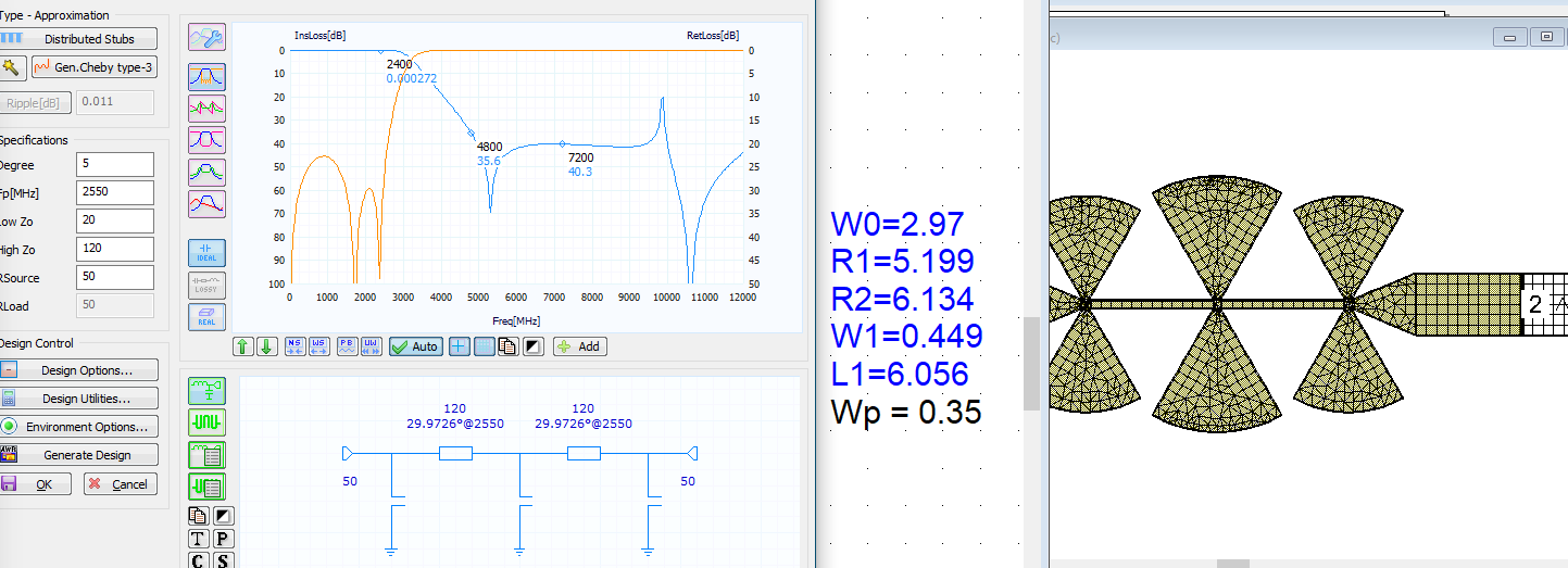
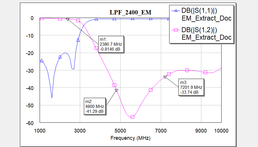
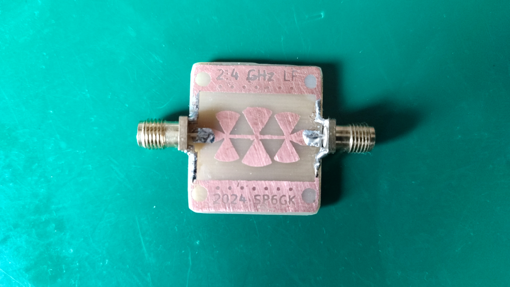
This is a distributed stub low-pass filter based on a Chebyshev Type 3 polynomial. The desired cutoff was set to 2.55 GHz so that it can be placed after a 2.4 GHz amplifier or mixer.

Couplers and combiners

Two stage Wilkinson divider

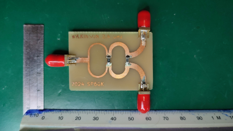
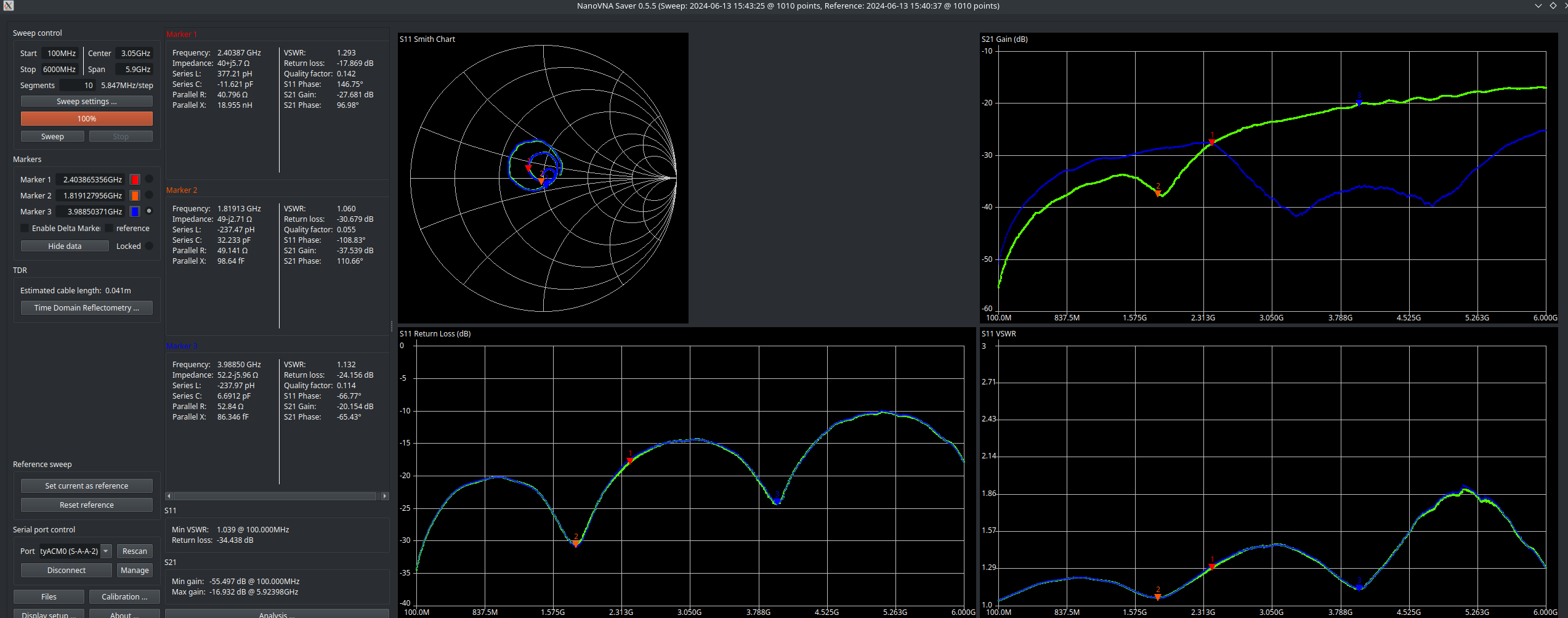
This 50/50 divider was designed for a center frequency of 2.4 GHz. Two stages are used to increase the fractional bandwidth. This is an early design, so I used a 1.6 mm PCB, resulting in thick traces. For a lower-order Wilkinson divider, the thickness of the traces is usually not a problem. However, if you want to design a four-stage Wilkinson divider or more, you will realize that the stages close to the input port are very thin, while the traces close to the output ports are quite wide. LitleVNA 64 was used to evaluate the design. Since this is a broadband divider designed for 2.45 GHz the maximum frequency span was set to 5 GHz with start frequency of 1 GHz. VNA was calibrated for this range with 404 points of measurements. The following plots were made using VNA-Saver, marker was set to 2.45 GHz. Because used VNA has only one port that can measure return loss and one port for insertion loss, during the measurement one output of the divider was terminated with 50 Ω load, then trace was saved as reference and then ports were swapped.

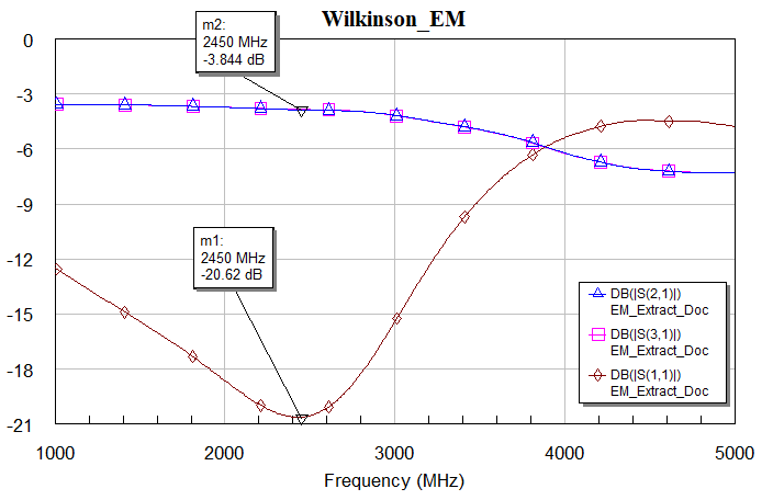
It can be seen that both ports have very similar transmission and even slightly better insertion loss than simulation has predicted -3.68 dB instead of -3.84 dB. It can also be seen that the divider maintains equal division but the insertion loss is significantly higher above 2.7 GHz. It was also observed that the return loss at 2.45 GHz is excellent -30 dB. This is also better than simulation however it appears to degrade faster. The match is still acceptable from 1 GHz to 3 GHz which is thanks to multiple section implementation. It can be concluded that the home made PCB gives results extremely close to the EM simulation. Largest disadvantage of this divider is its insertion loss. Phase measurement was omitted since Wilkinson is not a quadrature divider.

30 dB directional coupler

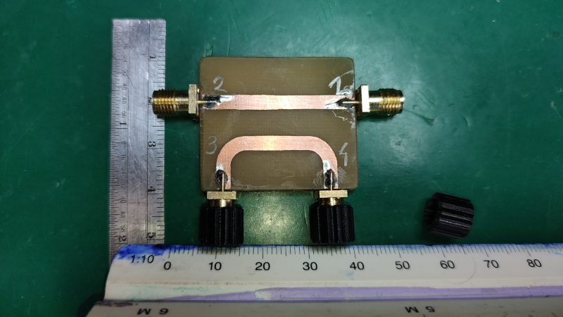
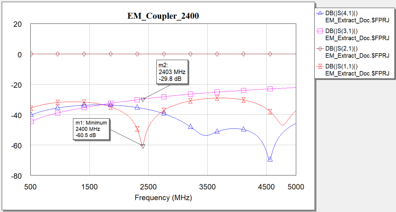
I designed this simple directional coupler to safely sample the output from 2.4 GHz power amplifiers. One port has to be terminated in a 50 Ohm load however, this also allows the use of a detector to measure reflected and forward power. The coupler was designed for a 1.6 mm FR4 PCB with 0.35 μm copper. I ran out of the 1.6 mm FR4 when etching this board, so I used a 2.0 mm thick laminate, and it still works well even though the trace should be thicker. In reality, if you make such a coupler with a controlled impedance trace, the return loss should be somewhat better.

Compact branchline hybrid

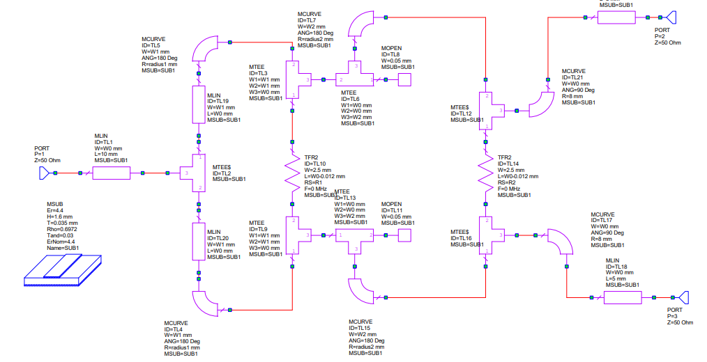
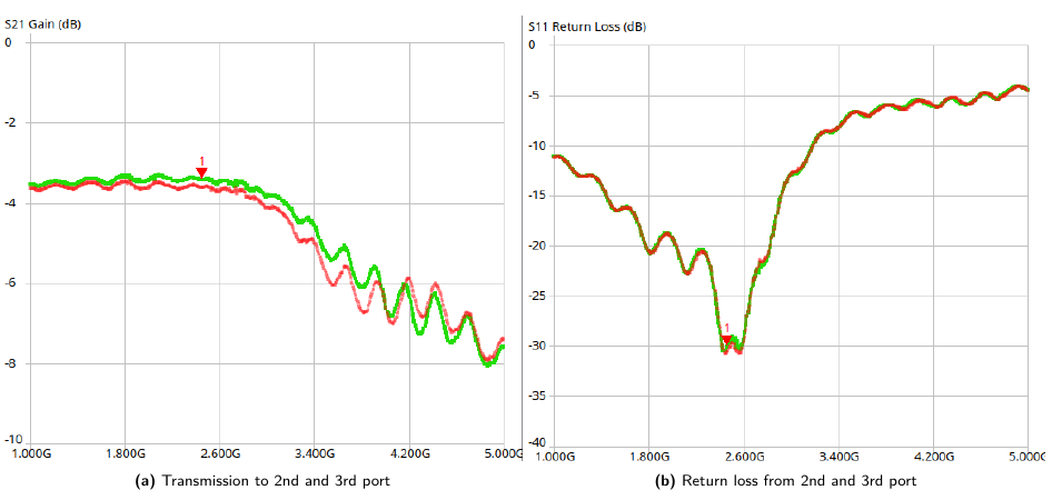
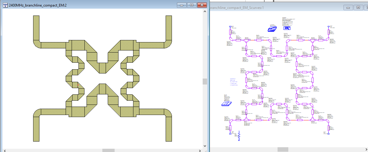
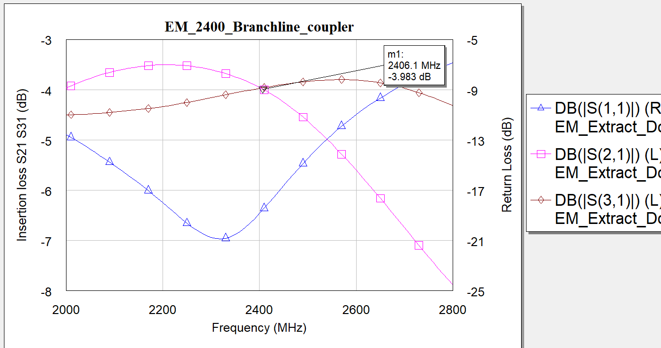
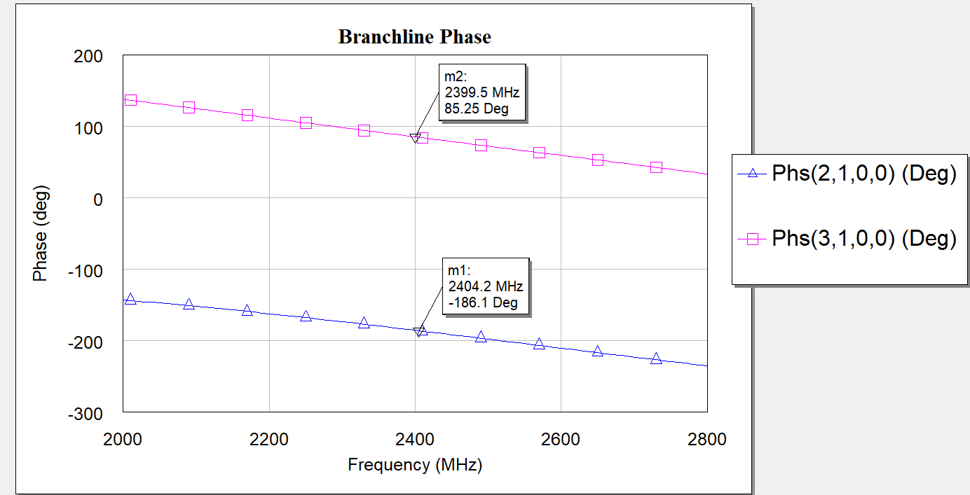
This is a branchline coupler with folded transmission lines to minimize the footprint. It works well in EM simulation, but I have yet to etch and measure it on a real laminate. At some point, I would like to design a balanced amplifier. Such configurations require the use of couplers that split and combine signals with a 90-degree phase difference, and a branchline coupler is one way to achieve this. Here the phase shift is not ideal, but the footprint is smaller than 15x16 mm. The S31 and S21 parameters are practically identical in EM simulation at the design center frequency, which is good. These values would ideally be -3 dB, but there is also some inherent loss in the traces of the hybrid. One can also notice that this circuit is rather narrow, maintaining good amplitude balance at a single point; therefore, this hybrid will be used in a tuned balanced amplifier.